Lab 5: Databases

Overview

In this lab, you will be learning about relational database systems through activities in Postgres.

To receive credit for this lab, you MUST show your work to the TA during the lab, and push it to the github before the deadline. Please note that submissions will be due on Wednesday at 11:59 p.m. in the following week.

Learning Objectives

LO1. Learn to read and construct ER diagrams
L02. Understand the basics of Data Definition Language (DDL)
L03. Use SQL to query and modify tables
L04. Learn to use more advanced SQL features like CTEs, Group By, and Joins

Part A

Pre-Lab Quiz

Complete Pre-Lab quiz on Canvas before your section's lab time.

Part B

ER Diagram

What is an ER diagram?

An entity-relationship (ER) diagram is a blueprint that shows how "entities" such as people, things, and concepts are related to each other in a system. ER diagrams are most commonly used to design or debug relational databases in software development, business informatics, education, and research. Also known as ERD or ER model, it uses a predefined set of symbols such as rectangles, diamonds, ellipses, and connecting lines to represent the interconnectivity of entities, relationships, and their attributes.

Below is the ER Diagram for the database that we will be using for this lab. Please refer to it while writing queries in the later portion of the lab.

🎥Recording output

Nothing to be recorded here.

Directory Structure

NO GenAI usage

For this lab, we do not prescribe the usage of Gen AI tools. Please attempt this lab by yourself. If you choose to use Gen AI, follow the guidelines in the syllabus or from the GenAI section in Lab 1 to appropriately cite your usage. Failure to do so will result in a 0 on the entire lab.

Clone your GitHub repository

info

You need to accept the invite to the GitHub classroom assignment to get a repository.

Github Classroom Assignment

For the next two steps, make sure to edit the name of the repository after the copying the command into your terminal.

Using an SSH key
Using a Personal Access Token (PAT)

git clone git@github.com:CU-CSCI3308-Fall2025/lab-5-databases-<YOUR_USER_NAME>.git

git clone https://github.com/CU-CSCI3308-Fall2025/lab-5-databases-<YOUR_USER_NAME>.git

Navigate to the repository on your system.

cd lab-5-databases-<YOUR_USER_NAME>

The website directory structure contains the SQL files for this lab. The list below contains all the files that are provided and the ones you will submit as well. Please make sure to follow the guidelines specified here.

├── data
│   ├── actors.sql
│   ├── genres.sql
│   ├── movies_to_actors.sql
│   ├── movies_to_genres.sql
│   ├── movies.sql
│   └── platforms.sql
├── entrypoint.d
│   ├── 00_create.sql
│   ├── 01_alter.sql
│   ├── 02_insert.sql
│   ├── 03_verify.sql
│   ├── 04_insert.sql
│   └── lab5_ec_persist.sql  (Extra Credit)
├── queries
│   ├── query_01.sql
│   ├── query_02.sql
│   ├── query_03.sql
│   ├── query_04.sql
│   ├── query_05.sql
│   ├── query_06.sql
│   ├── query_07.sql
│   ├── query_08.sql
│   ├── query_09.sql
│   ├── query_10.sql
|   ├── lab5_ec_load.sql (Extra Credit)
|   └── EC_analysis.txt (Extra Credit)
├── docker-compose.yaml
└──  README.md

Initializing Docker Container

In your repository, you will find a docker-compose.yaml file with the following contents:

docker-compose.yaml
services:
  db:
    image: 'postgres:14'
    env_file: .env
    expose:
      - '5432'
    volumes:
      - postgres-data:/var/lib/postgresql/data
      - ./data:/data:ro
      - ./entrypoint.d/:/docker-entrypoint-initdb.d:ro

volumes:
  postgres-data: {}

Create a .env file in the root (lab5-sql-\<your_username>) folder to store environment variables to setup postgres.

.env
# database credentials
POSTGRES_USER="postgres"
POSTGRES_PASSWORD="pwd"
POSTGRES_DB="movies_db"

You should not commit this file to GitHub (it is in the .gitignore file, so this is automatic.)

Start the PostgreSQL docker container with the docker-compose.yaml file:


docker compose up -d

Now that the container is running in the background, connect to PostgreSQL shell:

docker compose exec db psql -U postgres

PostgreSQL

Connect to the movies database


\c movies_db;

Here is a list of some useful terminal commands for PostgreSQL that you will need for the later tasks in the lab.

To list all of the databases in the current PostgreSQL database server, use the \l command

\l

To list all of the tables in the current database, use the \dt command

\dt

To describe a table such as the column, type, modifiers of columns, etc., use \d followed by the table name like so


\d table_name

To view all of the data associated with a table, select all of the columns from a table like this:

SELECT * FROM table_name;

To display the command history, use the \s command

\s

Comments

Single line comments start with --, while multi-line comments start with /* and end with */. Any text between /* and */ will be ignored while executing the .sql files. Use multi-line comments to include formatted query outputs in sql files.

Example:

-- Select all the columns of all the records in the Customers table:

SELECT * FROM customers;
/*
| customer_id | customer_name |
|    123      |    David      |
*/

A. Data Definition Language (DDL)

A.1. CREATE table

Creating the tables

To actually create a table we must start with the "CREATE TABLE" command. Follow this with the name of the table you want to create. To make sure the script is re-runnabe you should use "IF NOT EXISTS" [CREATE TABLE IF NOT EXISTS table_name] to your script to ensure postgreSQL doesn't try to recreate a table (handy when working with long/reused scripts).

PLEASE NOTE: While the commands are demonstrated here in uppercase, postgreSQL is NOT case sensitive. It is convention to list the postgreSQL commands in upper case.

Syntax:

CREATE TABLE table_name (
  column_name1 DATATYPE,
  column_name2 DATATYPE
);

Example:

Following is an example of the CREATE TABLE command.

caution

DO NOT MAKE THIS TABLE. Use this as a guide to create the necessary tables.

/* Create a table names products with the mentioned columns
having the datatypes mentioned */
CREATE TABLE products (
  product_id SERIAL PRIMARY KEY /* the primary key for each entry */,
  product_name VARCHAR(200) NOT NULL,
  quantity_per_unit VARCHAR(20),
  unit_price FLOAT,
  units_in_stock SMALLINT,
  units_on_order SMALLINT,
  reorder_level SMALLINT,
  discount DECIMAL,
  category_id SMALLINT
);

caution

Just about every postgreSQL command ends with a semicolon. If you don't add one, then the terminal will simply wait until you enter it. MAKE SURE TO ADD YOUR SEMICOLONS!

The table will look something like this with no data inserted.

product_id	product_name	quantity_per_unit	unit_price	units_in_stock	units_on_order	reorder_level	discount	category_id

You may have noticed certain keywords in the query such as SERIAL, PRIMARY KEY and NOT NULL. Here are some definitions for your reference.

SERIAL

The SERIAL command creates an auto-increment that is managed by the database. Each time a new entry is added to the table, the SERIAL column is set and the value is incremented by 1

PRIMARY KEY

The PRIMARY KEY defines a unique identifier for each row of the table. THIS MUST BE A UNIQUE VALUE! This is how the database differentiates the various rows/entries of the table.

NOT NULL

The NOT NULL attribute requires that a field be set when a new entry is added to the table. This is a design choice, so only set a field to NOT NULL, when you really want to ensure that data is entered. For example, the slogan field does not have "NOT NULL" listed. Meaning that you can add a new item to the store table and skip the slogan field, but must provide a name, qty, and price.

Data Types

You can find the official documentation that lists all of PostgreSQL's supported data types here.

VARCHAR(#)

A variable-length character string, where # defines the maximum number of characters. This is a go-to option for defining strings that need to be set a maximum length. As a note, make sure to use single quotes ' ' when working with VARCHAR data.

TEXT

The TEXT type is fairly similiar to the VARCHAR(#) data type, but removes the character limit.

Whole Numbers

Whole numbers, or integers, can come in various sizes (smallint, int, and bigint). You should choose which one to use based on the specific data you hope to store.

Name	Number of Bytes	Range	Recommended Use
smallint	2	-32,768 to 32,767	Only use when you KNOW your values won't exceed its range (ex. the height of a person in inches or the age of a person in years)
int or integer	4	-2,147,483,648 to 2,147,483,647	Considered the "work-horse" data type and most often used for giving you a good balance between range and data storage.
bigint	8	-9,223,372,036,854,775,808 to 9,223,372,036,854,775,807	Only use when you KNOW you are dealing with very large values (ex. number of transactions Amazon handles in a year).

Decimal Numbers

Decimal Numbers come in three different option - real, double precision, and numeric(#, #). Like the whole numbers above, the type you use depends on what kind of information you hope to store.

Name	Precision	Recommended Use
real	6 Decimal Places	Having up to 6 Decimal Places, means that real will work for "most cases" when dealing with decimal numbers.
double precision	15 Decimal Places	Use when you're dealing with scientific data or small decimal information.
numeric(precision, scale)	precision defines the total number of digits in a value scale defines the number of decimal places in a value Example: 12345.67 - this value has a precision of 7 (7 total digits) and a score of 2 (2 decimal places)	Use this when you are dealing with currencies or other data that requires a maximum number of digits. According to the documentation: Numeric values are physically stored without any extra leading or trailing zeroes. Thus, the declared precision and scale of a column are maximums, not fixed allocations.

DATE

Date values, in postgreSQL, are in the yyyy-mm-dd format - '2019-11-25'. To work with dates, see the list of handy date functions below:

Function Name & Example	Function Description
to_date(date_text, date_format)	The to_date() function will convert a string literal into a date value, using the provided date formate. Further details here.
to_date('20191125', 'yyyymmdd')
NOW():: DATE	To retrieve the current date on the server you can use the NOW() function, with the :: DATE option added to it we will only get the current date (removes the time information). The other option is to retrieve the CURRENT_DATE which will is in the default format of 'yyyy-mm-dd'.
SELECT NOW()::DATE
CURRENT_DATE
SELECT CURRENT_DATE;
Further Examples	If you want to learn more about working with dates, check out this resource here.

To Do - Create tables in movies DB

For this activity, you will be using the file entrypoint.d/00_create.sql.

tip

It would be easier for you to write your CREATE queries in this file before executing them on the terminal.

You need to choose suitable datatypes for the columns and identify and assign primary keys in the tables. You may refer to the ER diagram provided at the top of this page for this activity.

caution

Make sure you are connected to the movies database.

tip

Please refer the ER Diagram above to understand the datatypes for the necessary variables.

Create movies table with the following columns:
Note: Do not assign a foreign key relationship between the platform_id column of this table with the id of the platforms table. We will do that in the next section.
id
name
duration
year_of_release
gross_revenue
country
language
imdb_rating
platform_id
Create actors table with the following columns
id
name
agency
active_since
location
Create platforms table with the following columns
id
name
viewership_cost
Create genres table with the following columns
id
name
Create movies_to_actors table with the following columns
movie_id
actor_id
Create movies_to_genres table with the following columns
movie_id
genre_id

info

Multi-line Comments: Multi-line comments start with /* and end with */. Any text between /* and */ will be ignored while executing the .sql files.

Example:

/* Select all the columns
of all the records
in the Customers table: */

SELECT * FROM Customers;
/*
| customer_id | customer_name |
|    123      |    David      |
*/

File name: entrypoint.d/00_create.sql This file should include the CREATE queries and the outputs of the commands in this file.
The outputs copied in the entrypoint.d/00_create.sql file should be commented out using Multi-line comments. (/* */) as shown above.

A.2. ALTER table

There could arise scenarios that need you to alter the structure of table. This could mean adding/updating/deleting a column/constraint. In such situations,we make use of the ALTER TABLE command.

Syntax:

ALTER TABLE table_name
ADD COLUMN new_column_name data_type constraint;

Example:

/* Alter the table products to change the constraint
of foreign key to category_id column */
ALTER TABLE products
ADD CONSTRAINT category_id FOREIGN KEY (category_id) REFERENCES categories (category_id);

To Do - Alter Table

For this activity, you will be using the file entrypoint.d/01_alter.sql.

tip

It would be easier for you to write your ALTER queries in this file before executing them on the terminal.

Make the column platform_id a FOREIGN KEY in the movies table. You need to determine which column from which table this column would reference.

🎥Recording output

File name: entrypoint.d/01_alter.sql. This file should include the ALTER query and their outputs.
The outputs copied in the entrypoint.d/01_alter.sql file should be commented out using Multi-line comments. (/* */) as shown above.

A.3. DROP table

In case you want to get remove a table or in other words delete a table - DROP TABLE is the command to use.

caution

Please be very careful when using the DROP command because it will erase the table, the data within the table and all the metadata associated with that table.

Syntax:

DROP TABLE IF EXISTS table_name;

Example:

DROP TABLE IF EXISTS products;

Cascade is used to remove the specified records and foreign keys referencing them in other tables.

🎥Recording output

Nothing to record and output here.

tip

TROUBLESHOOTING

To stop and remove all containers, networks, and volumes created by Docker Compose, you can use:

docker compose down -v

down stops and removes the running containers and networks created by your Compose file
-v ensures that any named or anonymous volumes created by the services are also removed

This is useful if:

You want to reset your environment from scratch
Something has gone wrong with persistent data (e.g., a database volume got corrupted)
You want to ensure no leftover data is influencing the next run

However, running with -v will permanently delete all data stored in your containers’ volumes, so be careful!!!!

B. Data Manipulation Language (DML)

B.1. INSERT INTO table

Insert Provided Data

You will now insert rows from the provided sql files under data in your repository We mounted the data folder in your repository to /data in the container. In your postgres terminal, type a command to insert rows for each table; replace <filename> with the actual file name for each table.

\i /data/<filename>.sql;

🎥Recording output

Add each of the 6 commands and their output to entrypoint.d/02_insert.sql.

Verify that the data was correctly inserted. Replace <table_name> with each table.

select count(*) from <table_name>;

Tables and expected number of rows in each table

Table Name	No. of Rows
Movies	26
Actors	20
Platforms	7
Genres	8
movies_to_actors	61
movies_to_genres	26

info

Multi-line Comments: Multi-line comments start with /* and end with */. Any text between /* and */ will be ignored while executing the .sql files.

Example:

/* Select all the columns
of all the records
in the Customers table: */

SELECT * FROM Customers;
/*
| customer_id | customer_name |
|    123      |    David      |
*/

🎥Recording output

1. Copy the verification queries and their outputs to show the number of rows in each table to a file. You must use /* */ to comment out the outputs of the verification queries.

File name: entrypoint.d/03_verify.sql

Now let's practice inserting some new rows of our own

The INSERT query will add records to the table.

Syntax:

INSERT INTO table_name (column_name1, column_name2, column_name3,...column_nameN)
  VALUES (value1, value2, value3,...valueN), /* First row  */
  (value1, value2, value3,...valueN);        /* Second row */

Example:

/* Insert the values into corresponding columns in the table products */
INSERT INTO products (product_name, quantity_per_unit,  unit_price, units_in_stock, units_on_order, reorder_level, discount, category_id) VALUES
  ('Unison Composition Book', '3',  10.4, 100, 50, 2, no, 1);

Insert with return inserted row

The "returning *" clause at the end of the query will return all columns for the newly inserted record.

INSERT INTO products (product_name, quantity_per_unit,  unit_price, units_in_stock, units_on_order, reorder_level, discount, category_id) VALUES
  ('Unison Composition Book', '3',  10.4, 100, 50, 2, no, 1) returning * ;

To Do - You should insert at least 2 rows in each table. (The data should satisfy the constraints on the tables).

For this activity, you will be using the file entrypoint.d/04_insert.sql.

tip

It would be easier for you to write your INSERT queries in this file before executing them on the terminal.

info

Multi-line Comments: Multi-line comments start with /* and end with */. Any text between /* and */ will be ignored while executing the .sql files.

Example:

/* Select all the columns
of all the records
in the Customers table: */

SELECT * FROM Customers;
/*
| customer_id | customer_name |
|    123      |    David      |
*/

🎥Recording output

File name: entrypoint.d/04_insert.sql This file should contain all INSERT queries and their outputs. The outputs copied in the entrypoint.d/04_insert.sql file should be commented out using Multi-line comments. (/* */) as shown above.

B.2. UPDATE table data

More often than not, there can be a need to update the data in a table. For that purpose, we can use UPDATE table command. You need to make sure to specify a condition, using the WHERE clause when you update rows in a table otherwise all the rows in the table will be updated. We'll learn more about the WHERE clause in the querying section of this lab.

Syntax:

UPDATE table_name
SET column1 = value1,
    column2 = value2,
    ...
WHERE condition;

🎥Recording output

Nothing to record here

B.3. DELETE table data

In some cases you may need to remove a row from the table. DELETE is the command to use. Similar to the UPDATE command, you need to make sure to specify a condition, using the WHERE clause when you update rows in a table otherwise you may end of deleting all the rows in the table. We'll learn more about the WHERE clause in the querying section of this lab.

Syntax:

DELETE FROM table_name
WHERE condition;

🎥Recording output

Nothing to record here

C. Data Query Language (DQL)

C.1. Basic Queries

In this section we will learn some important commonly used queries in the premise of products database seen previously.

SELECT Statement

Used to select and display rows of data from table.

Syntax:

SELECT column_name FROM table_name WHERE condition_is_true;

Select Everything:

The asterisk (*) or "star" acts as a wild card in our select statement. When we don't want to limit the number of fields/columned returned we can use * to select all of them.

Example:

/* SELECT all the rows from table products */
SELECT * FROM products;

The FROM statement defines where we want to retrieve our data (this is usually a table name, but could also be a view or even a subquery).

Limit Our Columns:

If we want to choose and display only selected columns instead of all columns, we can do so by the following way.

Example:

/* Only show the product_name and quantity_per_unit columns from table products. */
SELECT product_name, quantity_per_unit FROM products;

In the above example, product_name and quantity_per_unit are the names of columns that we are choosing to display out of the many columns that might be present in the table products. This is great when we have large tables with a large number of rows or when we want to display columns side-by-side for improved readability.

Limit Our Rows:

If we want to select only some rows based on one or more conditions, we can use where clause. This clause helps us limit the number or rows returned. This is a true/false boolean statement that the database evaluates for each row. If the row evaluates to true, its information is returned. Otherwise the row is skipped over/ignored.

Example:

/* Show the rows in columns product_name, quantity_per_unit in table
products where unit_price is less than 1 dollar*/
SELECT product_name, quantity_per_unit FROM products WHERE unit_price < 1;

Aliases

Basic Syntax

SELECT column_name AS alias_name FROM table_name as table_alias_name;

Rename A Column

 SELECT item_name, qty AS quantity FROM store;

AS alias_name: Sometime our columns have short or abbreviated names (like qty). To help improve readability when we run our queries, we can use an alias to temporarily rename our column. In this example we are altering qty to the complete word quantity. But what if we wanted to work with multiple words? Then we can also place our alias in double quotes: qty as "Quantity of Items in Stock".

Rename A Table

 SELECT item_name, qty FROM store as retail_establishment;

AS table_alias_name: Aliases can also be applied to tables, but we don't usually do it for making our readouts more readable. Instead these are uses for helping us handle subqueries and joins. We'll cover these use cases in the next section.

Combining Fields

 SELECT item_name || ' : ' || slogan AS catch_phrase FROM store WHERE slogan IS NOT NULL;

item_name || ' : ' || slogan: The last option we'll discuss for using aliases is to help us rename concatenated or calculated fields. We use the double pipe || for string concatenation in SQL. So this statement states that we will be concatenating the item_name column and slogan columns, with a colon in between. The where clause was added to remove the rows that lack a slogan.

COUNT

The COUNT() function will return the number of rows that match a query.

COUNT(*)

Our first example is a quick way to check how many rows are in a table (a great way to see if an insert statement or query worked correctly!). The second example will incorporate a where clause, letting us now how many rows meet a specific condition.

Example:

/*count the number of rows in the products table */
SELECT COUNT(*) FROM products;
/* count the number of products that cost more than 1 dollar */
SELECT COUNT(*) FROM products WHERE unit_price > 1;

COUNT(product_id)

If a column name is listed inside of the COUNT() function, then rows with null fields will be ignored. In our now updated examples, we list the slogan column (which can be null). This means all of rows without a product_id are completely ignored by the COUNT() function.

Example:

/*count the number of products in the products table which have a product_id*/
SELECT COUNT(product_id) FROM products;
/* Count the number of products that cost more than 1 dollars */
SELECT COUNT(product_id) FROM products WHERE unit_price > 1;

COUNT(DISTINCT prices)

By adding the DISTINCT keyword, we can limit our search to ignore duplicates. In this example, Gold Fish & Pringles share the same price, so collectively they only count as 1 entry! Use DISTINCT to help you determine how varied your table data is. Ignore Null & Duplicates

Example:

/*Count the number of rows with product_id which have unique values */
SELECT COUNT(DISTINCT product_id) FROM products;
/* Count the number of rows in the products table which have unique non-null prices that are above 1 dollar. */
SELECT COUNT(DISTINCT product_id) FROM products WHERE unit_price > 1;

SUM

The SUM() function will add up all of the numeric values in a column and return their combined sum. Just like COUNT(), we can apply a WHERE clause to limit which rows we add together. As a note, this will ignore null entries.

All Rows

Example:

/*Sum up the quantity_per_unit column*/
SELECT SUM(quantity_per_unit) FROM products;

Subset of Rows

Example:

/* Sum up the total quantity_per_unit for items that cost more than 1 dollar*/
SELECT SUM(quantity_per_unit) FROM products WHERE price > 1;

Math Operations

A complete list of operations can be found in the official documentation here. Use the table listed below for our Math Operations Examples

Addition

SELECT product_name, (units_in_stock + units_on_order) as "Total future stock" from products;

(units_in_stock + units_on_order): Working with the plus sign, we can add the values of two columns together for each table entry. For example, adding the units currently in stock and units ordered from the seller will give us the future total stock.

Subtraction

SELECT product_name, (units_in_order - reorder_level) as "Units to be sold before reorder" from products;

(units_in_order - reorder_level): Working with the minus sign, we can subtract the values of two columns from one another for each table entry.

Division

SELECT product_name, (unit_price / quantity_per_unit) as "Unit Price by quantity per unit" FROM products;

CAST (...): Our math operations will try to perserve the data type of the columns being used. This means if our operation works with whole numbers, then our answer will be a whole number. To work around this, we can use CAST() to treat one of our values as a float, which will result in a decimal number for our answer!

Multiplication

SELECT product_name, (units_in_stock* quantity_per_unit) as "Total amount in stock" FROM products;

((...)* 100): Like many other programming langauges, we can use the asterisk to handle multiplication. In this case we are multiplying with a constant 100.

GROUP BY

Basic Syntax

/*Use SUM to aggregate over column 2 */
SELECT column_1, SUM(column_2)
FROM products
/* Make groups keyed by column 1 values, that sum over column_2 */
GROUP BY column_1;

GROUP BY column

When we want to summarize sets of rows that share values, the GROUP BY statement is often useful. When coupled with an aggregate function like SUM or COUNT, we can aggregate values by groups. For example, if our products had a category column, we could sum the qty within each category, like fruit. For example:

Example:

/* select category_id and sum of units in stock grouped by category_id from table products */
/* This means that all proucts having same category_id are put in the same group and each group's units_in_stock is summed up */
SELECT category_id, SUM(units_in_stock)
FROM products
GROUP BY category_id;

GROUP BY HAVING column

The HAVING clause is used to filter groups returned by the GROUP BY clause. It is particularly useful when you want to include conditions on aggregated data, such as sums, averages, counts, etc., that cannot be filtered through the WHERE clause. For example:

Example:

/* select category_id and sum of units in stock grouped by category_id from table products */
/* This means that all proucts having same category_id are put in the same group and each group's units_in_stock is summed up */
/* Only include groups where the sum of units_in_stock is greater than 100 */
SELECT category_id, SUM(units_in_stock)
FROM products
GROUP BY category_id
HAVING SUM(units_in_stock) > 100;

C.2. Views, Subqueries and CTEs

Working With Views :

Syntax

CREATE VIEW view_name as your_query_goes_here;

Create View

A VIEW works with a pre-defined query and creates a resulting table. The view's fields can be accessed in the exact same way as a normal table. This is a handy way to aggregate data into more easy to access table format. Also, if you find yourself reusing query over and over, make it into a view for easier access.

Example:

CREATE VIEW inventory_cost AS
  SELECT product_name, (units_in_stock * unit_price) AS "Total Cost"
  FROM products;

Access a View

Example:

SELECT *
FROM inventory_cost /* Retrieve all of the rows from inventory_cost's query */;
SELECT * FROM inventory_cost WHERE "Total Cost" > 12;
/* Restrict the rows returned to only those with an inventory cost greater than 12 dollars  */

SUBQUERIES

A subquery can allow you to run an inner query that feeds its results into an outer query. Often this is utilized in the WHERE clause of a select statement to help define which rows a query should work with.

In our example above, our subquery will retrieve the current price of a Kit Kat. This means we don't have to worry about "hard coding" the price for a Kit Kat. Our outer query will always work, even if the price of a Kit Kat is updated.

Example:

/* Display all of the product items that have a price greater than a Kit Kat */
SELECT *
FROM products
WHERE
  unit_price > (SELECT unit_price FROM products WHERE product_name = 'Kit Kat');

CTE - Common Table Expressions

CTE is a temporary names result-set created using with and select clause. You can use this temporary result to further select, insert, update or delete. This is a convenient way to manage complex queries. We give a temporary name to the CTE which acts like a View. In the following syntax, temp_cte is the name of the intermediate view which has columns a,b,c selected from table1. This view is further used to select a and c columns where b's value is greater than 3.

Syntax

WITH
  temp_cte AS (
    SELECT a, b, c
    FROM table1
  )
SELECT a, c
FROM temp_cte
WHERE b > 3;

Building on the previous exmaple of displaying all products that have a price greater than KitKat, let's use CTE to do the same.

Example:

/* Display all of the product items that have a price greater than a Kit Kat */
WITH
  kit_kat_price AS (
    SELECT price
    FROM products
    WHERE name = 'Kit Kat'
  )
SELECT name, price
FROM products
WHERE price > (SELECT price FROM kit_kat_price);

This query creates a temporary result-set named kit_kat_price that returns the price of the product named 'Kit Kat'. Then, in the main query, we select the name and price of all products where the price is greater than the price of 'Kit Kat'.

C.3. Joins

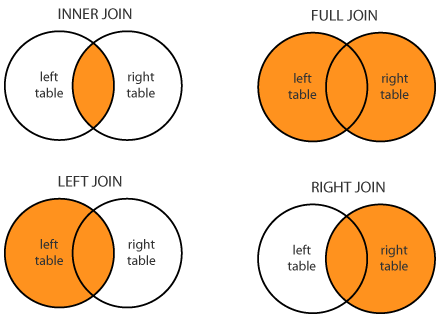
You can find a more detailed explanation of Joins for PostgreSQL here.

Checkout the handy diagram below:

index

Example:

Consider the following tables for performing joins. We will be using the employee table on the left and salary table on the right of the join condition for the purpose of this explanation.

CREATE TABLE employee (
  id SERIAL PRIMARY KEY,
  name VARCHAR(60) NOT NULL,
  age INT NOT NULL,
  phone_number VARCHAR(10) NOT NULL
);

INSERT INTO employee
  (name, age, phone_number)
VALUES
  ('Randolph Esquire', 33, '1112223333'),
  ('Clarence Roosevelt', 12, '4442220000'),
  ('Rachel Null', 44, '1002004000'),
  ('Sarah The Third', 102, '1032034003');

-- --

CREATE TABLE salary (
  employee_id INT PRIMARY KEY,
  starting_salary FLOAT NOT NULL,
  current_salary FLOAT NOT NULL
);

INSERT INTO salary
  (employee_id, starting_salary, current_salary)
VALUES
  (1, 35000, 37222.32),
  (2, 55.33, 78.92),
  (3, 123450.12, 277111.32),
  (5, 100, 323.5);

index

info

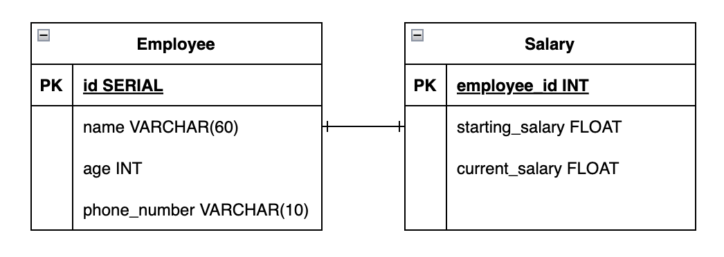
Any blank cells that you see in the answer sets, are NULL values.

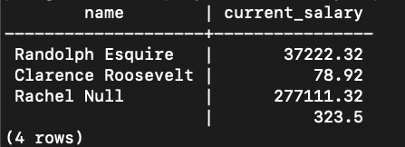
INNER JOIN

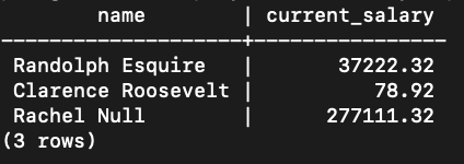
The INNER JOIN will return only the entries that have matching values in a shared column, in this case a shared column between the "employee" & "salary" tables is id <-> employee_id. By default, if you do not specify the type of join, the JOIN keyword in SQL will refer to an inner join.

Example:

Command:

SELECT
  employee.name,
  salary.current_salary
FROM
  employee -- left table
  INNER JOIN salary -- right table
    ON employee.id = salary.employee_id;

Output:

You'll see that "Sarah the Third" is an entry with in the employee table with id = 5. Since there isn't an entry in the salary table with employee_id = 5, that entry is left out.

index

LEFT JOIN

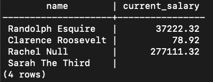
The LEFT JOIN works similarly to the inner join, except ALL rows from the left table are returned. The fields from the right table will either be set to NULL, or to the value from the right table if there is a match. This means you will see null values for some fields from the right column in the cases that there was no match.

Example:

Command:

SELECT
  employee.name,
  salary.current_salary
FROM
  employee -- left table
  LEFT JOIN salary -- right table
    ON employee.id = salary.employee_id;

Output:

index

RIGHT JOIN

The RIGHT JOIN works the same as the left join, but opposite. That is, ALL rows from the right table are returned. The fields from the left table will either be set to NULL, or to the value from the right table if there is a match.

Example:

Command:

SELECT
  employee.name,
  salary.current_salary
FROM
  employee -- left table
  RIGHT JOIN salary -- right table
    ON employee.id = salary.employee_id;

Output:

index

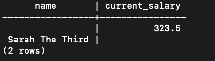
FULL JOIN

Example:

The FULL JOIN will return all the entries from each table that have matching pairs. For any entry that doesn't, it will display null for the field.

Command:

SELECT
  employee.name,
  salary.current_salary
FROM
  employee -- left table
  FULL JOIN salary -- right table
    ON employee.id = salary.employee_id;

Output:

In this example, the entry "5" and "Sarah The Third'' will be paired up with null values.

index

FULL JOIN - (rows that DON'T have matching pairs)

This is a variant of FULL JOIN in which it will only return the entries that DON'T have matching pairs (i.e. unique data entries). This means you will only see the rows that contain a null value on other side. (Entry "5" & "Sarah The Third")

Example:

Command:

SELECT
  employee.name,
  salary.current_salary
FROM
  employee -- left table
  FULL JOIN salary -- right table
    ON employee.id = salary.employee_id
WHERE employee.id IS NULL OR salary.employee_id IS NULL;

Output:

index

C.4. Querying data

For each query in this activity, you will be editing the corresponding file in queries.

Write a query to find the highest rated movie. If there is a tie, return any ONE row with the movie with the highest rating.

Hint: Start from the movies table. Sort the results by the imdb_rating column in descending order so the highest appears first. Use a clause to return only the first row.

Write a query to find ALL the movies starring "Leonardo di Caprio".

Hint: Use the join table that links movies and actors. Join movies, movies_to_actors, and actors. Then filter on rows where the actor’s name matches "Leonardo di Caprio".

Write a query to find the top 3 oldest movies in the database. Return only THREE rows.

Hint: Use the movies table. Sort rows by year_of_release in ascending order so the oldest comes first. Limit the number of results to 3.

Part C

Write a query to get movies available on Hulu ordered by id.

Hint: First identify Hulu’s platform id from the platforms table. Use this id to filter the movies table. Order the results by the movie id.

Write a query to find the actor who has acted in the maximum number of movies.

Hint: Use the join table movies_to_actors to count how many movies each actor has. Group the results by actor id, then sort by the count in descending order to find the maximum. Return the actor’s name.

Top 3 highest grossing thriller movies.

Hint: Use movies, movies_to_genres, and genres. Join them together so that you can filter by genre_name = 'Thriller'. Order the results by gross_revenue in descending order and restrict to 3 rows.

Update the platform for all 2004 movies to be Netflix.

Hint: First, identify Netflix’s platform_id from the platforms table. Then update the movies table, changing the platform id for all movies where year_of_release = 2004.

Which platform has the most number of movies?

Hint: Group the movies table by platform id and count how many movies are on each platform. Sort by the count in descending order. Join back to the platforms table to get the platform name with the largest count.

Which actor’s movies have generated the overall highest revenue?

Hint: Join movies, movies_to_actors, and actors. Group the results by actor and compute the sum of gross_revenue. Sort these sums in descending order and return the actor with the highest total.

Write a query to find actors from Missouri that starred in a Romcom and order them by name.

Hint: Break the problem into steps. First, find actors from Missouri by filtering the actors table and joining it with movies_to_actors. Next, find all Romcom movies by joining movies, movies_to_genres, and genres filtered by Romcom. Finally, combine these two results to get only Missouri actors who appeared in Romcoms, and order the names alphabetically.

🎥Recording output

Files: queries/*.sql These files should each contain 1 query. Any outputs should be commented out. will not be graded.

Extra Credit

Extra Credit Analysis.
- In a text file queries/EC_analysis.txt, discuss the performance of your queries from Part B - C.4 and Part C.
- For each query, explain why you chose the specific SQL constructs (e.g., joins, CTEs, subqueries) and how they impact performance.
- If you can think of alternative ways to write the same query, include those as well and discuss their potential performance differences in queries/lab5_ec_load.sql.
- This analysis should demonstrate your understanding of SQL performance considerations.
Persist Lab 4 Calendar events to Postgres (DDL + DML).
- Create a new database "Calendar" using the following command:
```
CREATE DATABASE calendar;
```
- Using the event fields from Lab 4’s Calendar app (event name, weekday, time, modality, location or remote URL, and attendees), design a relational table schema and add it to the Calendar database.
- Include constraints on the columns that make sense (e.g., non-nulls, reasonable uniqueness, and types that match the data).
- Then write SQL that:
  (a) creates the required table(s), and
  (b) inserts/updates/deletes rows that correspond to Create/Update/Delete actions from the Calendar app.
- Place your DDL/DML in entrypoint.d/ in a new file lab5_ec_persist.sql (for table creation, inserts/updates/deletes that mirror your UI actions).
- Make sure the columns you choose map cleanly to the Lab 4 form fields and interactions (Create Event, Update Event). (Lab 4)
- Include all the files for this extra credit activity in your submission folder for this lab.

Note for students:

Use the same event fields and behaviors described in Lab 4 (modal form, validations, modality-dependent location vs. remote URL, saving events, rendering event cards). Your SQL design should reflect those exact fields and interactions.

Submission Guidelines

Commit and upload your changes

1. Make sure you copy your files for submission into your local git directory for this lab, within a "submission" folder that you need to create.
2. Run the following commands at the root of your local git directory, i.e., outside of the "submission" folder.

git add .
git commit -m "add submission"
git push

You will be graded on the files that were present before the deadline. If the files are missing/not updated by the deadline, you could receive a grade as low as "Not attempted". This can be replaced by raising a regrade request once you successfully upload your work to Github.

Regrade Requests

Please use this link to raise a regrade request if you think you didn't receive a correct grade.

Grading specifications

Not attempted
- Student has not attempted the lab OR
- Student has not attended the lab without prior approval
Below Expectations - If any of the following conditions are met
- Part A
  - Quiz has not been attempted OR
  - Quiz has been attempted, but
    - The answer to the questions are partially correct
- Part B
  - Student has not attended the duration of the lab
  - Student's work was not reviewed by the TA
  - Student has not uploaded their work to the GitHub repository OR
  - Student has not uploaded one or more the required files OR
  - Files are not representative of the student's attempt at the activity
- Part C
  - One or more of the files are missing from the GitHub repository
  - All files are present in the GitHub repository, but
    - The files have incomplete answers OR
    - The answers to the questions are incorrect
Meets Expectations - if all of the specified conditions are met
- Part A
  - Quiz has been completed
  - Students have been able to demonstrate their understanding by answering all the questions on the quiz correctly
- Part B
  - Student should have attended the duration of the lab
  - Student's work should have been reviewed by the TA and attendance should be marked on Canvas
  - Student has uploaded their work to the submission folder in the GitHub repository
    - Once the lab is completed, the student can copy the contents into the submission folder
  - The .env file has been created with the correct credentials
  - DDL
    - CREATE
      - Student has written the queries to create all the tables
      - All the columns in the tables have appropriate data types and constraints
        This can be verified by checking the 00_create.sql in the entrypoint folder
    - ALTER
      - Student has written the alter query correctly to add a foreign key
        This can be verified by checking the 01_alter.sql in the entrypoint folder
  - DML
    - INSERT
      - Student has successfully inserted the data provided in the data folder
        This can be verified by checking the 02_insert.sql in the entrypoint folder
      - Student should have run SELECT queries to ensure that the correct number of rows were inserted into the tables
        This can be verified by checking the 03_verify.sql in the entrypoint folder
      - Student should have inserted at least 2 rows in each table of the database with data of their own
        This can be verified by checking the 04_insert.sql in the entrypoint folder
  - DQL
    - Student has written the SQL queries for the 10 queries and included their outputs in the respective files in the queries folder
Exceeds Expectations
- Persist to Postgres (DDL + DML)
  - Designed a clean relational schema that maps 1:1 to Lab 4 fields (event name, weekday, time, modality, location/remote URL, attendees) with appropriate types and constraints (e.g., NOT NULL, sensible CHECKs, uniqueness on a natural/business key or surrogate + unique composite).
  - Includes CREATE TABLE IF NOT EXISTS so DDL is idempotent (i.e., it does not create the table if it already exists).
  - Placed DDL in entrypoint.d/ and DML in queries/lab5_ec_persist.sql exactly as specified.
  - DML supports Create/Update/Delete with correct mapping to UI actions (e.g., INSERT for Creating an event, UPDATE for Updating an event, DELETE for Deleting an event) and handles conflicts gracefully.
- Extra Credit Analysis
  - Provides queries/EC_analysis.txt explaining query choices (joins/CTEs/subqueries), and performance trade-offs.
  - Compares at least one alternative formulation for each query and discusses expected performance differences (e.g., CTE vs. views).

Overview​

Learning Objectives​

Part A​

Pre-Lab Quiz​

Part B​

ER Diagram​

Directory Structure​

Clone your GitHub repository

Navigate to the repository on your system.

Initializing Docker Container​

PostgreSQL​

Here is a list of some useful terminal commands for PostgreSQL that you will need for the later tasks in the lab.​

Comments​

A. Data Definition Language (DDL)​

A.1. CREATE table​

Example:​

VARCHAR(#)

TEXT

Whole Numbers

Decimal Numbers

DATE

To Do - Create tables in movies DB​

A.2. ALTER table​

To Do - Alter Table​

A.3. DROP table​

TROUBLESHOOTING​

B. Data Manipulation Language (DML)​

B.1. INSERT INTO table​

To Do - You should insert at least 2 rows in each table. (The data should satisfy the constraints on the tables).​

B.2. UPDATE table data​

B.3. DELETE table data​

C. Data Query Language (DQL)​

C.1. Basic Queries​

SELECT Statement​

Select Everything: ​

Example:​

Example:​

Example:​

COUNT​

Example:​

Example:​

Example:​

SUM​

Example:​

Example:​

Example:​

Example:​

GROUP BY​

Example:​

Example:​

C.2. Views, Subqueries and CTEs​

Working With Views :​

Syntax​

Create View​

Access a View​

SUBQUERIES​

CTE - Common Table Expressions​

Syntax​

Example:​

C.3. Joins​

Example:​

INNER JOIN​

Example:​

LEFT JOIN​

Example:​

RIGHT JOIN​

Example:​

FULL JOIN​

Example:​

FULL JOIN - (rows that DON'T have matching pairs)​

Example:​

C.4. Querying data​

Part C​

Extra Credit​

Submission Guidelines​

Commit and upload your changes​

Regrade Requests​

Grading specifications​

Overview

Learning Objectives

Part A

Pre-Lab Quiz

Part B

ER Diagram

Directory Structure

Initializing Docker Container

PostgreSQL

Here is a list of some useful terminal commands for PostgreSQL that you will need for the later tasks in the lab.

Comments

A. Data Definition Language (DDL)

A.1. CREATE table

Example:

To Do - Create tables in movies DB

A.2. ALTER table

To Do - Alter Table

A.3. DROP table

TROUBLESHOOTING

B. Data Manipulation Language (DML)

B.1. INSERT INTO table

To Do - You should insert at least 2 rows in each table. (The data should satisfy the constraints on the tables).

B.2. UPDATE table data

B.3. DELETE table data

C. Data Query Language (DQL)

C.1. Basic Queries

SELECT Statement

Select Everything:

Example:

Example:

Example:

COUNT

Example:

Example:

Example:

SUM

Example:

Example:

Example:

Example:

GROUP BY

Example:

Example:

C.2. Views, Subqueries and CTEs

Working With Views :

Syntax

Create View

Access a View

SUBQUERIES

CTE - Common Table Expressions

Syntax

Example:

C.3. Joins

Example:

INNER JOIN

Example:

LEFT JOIN

Example:

RIGHT JOIN

Example:

FULL JOIN

Example:

FULL JOIN - (rows that DON'T have matching pairs)

Example:

C.4. Querying data

Part C

Extra Credit

Submission Guidelines

Commit and upload your changes

Regrade Requests

Grading specifications